Principal Component Analysis

PCA is a dimensionality reduction technique used in data mining to get the most important features that best describe a data set. Because it can reduce the dimensions (i.e. features of the data), it aids in visualizing the behavior of the data.

The Math

PCA is a statistical interpretation of singular value decomposition (SVD). Its hugely reliant on the correlation between the dimensions of our data, more specifically the covariance matrix.

PCA is also a linear transformation.

The principal components (PCs) are linear combinations of the original features of the data. PCA is deeply dependent on the correlation between the features of a dataset.

To perform the linear transformation that will produce the eigs(the eigen values and their corresponding eigen vectors), we need to compute the covariant matrix. To do this:

1. Compute matrix B which is the mean-subtracted data
   $B = x - \overline{x}$
2. Create the covariant matrix which is a square matrix with dimension = the dimension of the original data.
   $\begin{bmatrix} var(x)&cov(x,y) \cr cov(x,y)& var(y)\end{bmatrix}$

For the purpose of this piece, we take our covariant matrix to be: $\begin{bmatrix}9&4\cr4&3\end{bmatrix}$

1. Perform linear transformation

  (x,y) ===> (9x + 4y, 4x + 3y)
  (0,0) ===> (0,0)
  (1,0) ===> (9,4)
  (0,1) ===> (4,3)
  (-1,0) ===> (-9,-4)
  (0,-1) ===> (-4,-3)

1. Compute the eigen vectors and the eigen values of the covariant matrix.
   $\begin{bmatrix}9&4\cr4&3\end{bmatrix} * v = \lambda * v$

$v$ = the eigen vector
$\lambda$ = the eigen value

1. The principal components are computed by multiplying the mean-subtracted data by the eigen vector of the covariant matrix
   $T = BV$
   $T$ = the principal components

2. T can also be calculated simply using SVD.
   $SVD(B) = U*\Sigma*V^T$
   $T = BV = U\Sigma$

$ U = V $ = eigen vectors
$B = \Sigma $ = eigen values

PCA WRT a Dataset

1. Say we have a data set with 5 dimensions.
   

   x1	x2	x3	x4	x5
   0	8	2	0	1
   3	5	1	8	9
   3	2	0	7	0
   3	3	0	2	6
   6	6	1	7	9
   5	6	1	8	0

import numpy as np
B = np.array([[0, 8, 2, 0, 1],
                [3, 5, 1, 8, 9],
                [3, 2, 0, 7, 0],
                [3, 3, 0, 2, 6],
                [6, 6, 1, 7, 9],
                [5, 6, 1, 8 0]])

1. Compute the covariance matrix of this dataset whose dimension is (5x5),
   

2. Compute the eigs of this matrix (in this case we’ll have 5 pairs of eigen vectors and values),
   $v_{1}, \lambda_{1}$
   $v_{2}, \lambda_{2}$
   $v_{3}, \lambda_{3}$
   $v_{4}, \lambda_{4}$
   $v_{5}, \lambda_{5}$

3. Rank the eigs based on the magnitude of the eigen values and pick the most important (the highest in magnitude) sets of eigs.
   

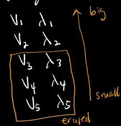
4. Choose the most important based on the eigen values ranked in descending order. For example, choosing the highest 2 enables us to visualize the data in a 2D plane.
   

PCR

PCR = PCA + a linear regression step that uses the method of least squares.

Usually in this linear regression step, you predict the value of a set target feature from the outcome of your PCs i.e. This target feature is not included in your feature sets at the time of the PCA analysis.